Dailysignalspk

Complete Binary Trees: Structure and Applications

Q: How are complete binary trees used in heap data structures?

Heaps, such as min-heaps and max-heaps, rely on complete binary trees to maintain a balanced and accessible priority structure. The completeness property ensures that insertions happen at the leftmost available position on the lowest level, preserving balance and enabling efficient operations like insertion and deletion.

Q: Why is array representation efficient for storing complete binary trees?

Complete binary trees can be efficiently stored in arrays because their nodes fill levels left to right without gaps, allowing parent and child relationships to be computed using simple index formulas. This eliminates the need for pointers, saving memory and improving cache efficiency.

Q: How do complete binary trees differ from full and perfect binary trees?

Complete binary trees require all levels except possibly the last to be fully filled with nodes aligned left to right, while full binary trees require every node to have either zero or two children. Perfect binary trees are both full and complete, with all levels fully filled. Complete binary trees offer more flexibility in the last level compared to the stricter full and perfect trees.

Q: What are common algorithms and operations performed on complete binary trees?

Common operations include insertion at the leftmost available position to maintain completeness, deletion by swapping the target node with the last node followed by re-balancing (heapify), and traversals such as inorder, preorder, postorder, and level order. These operations leverage the tree's structure for efficient performance, often with O(log n) time complexity.

Isabella Scott

13 May 2026, 12:00 am

Edited By

Isabella Scott

12 minutes of reading

Beginning

A complete binary tree is a specific type of binary tree with a distinct structure that makes it highly efficient for various computing tasks and algorithms commonly used in computer science. Unlike a generic binary tree where the leaf nodes can be scattered anywhere, in a complete binary tree every level, except possibly the last, is fully filled. The nodes on the last level are positioned as far left as possible. This layout leads to a well-organised, compact tree shape.

Understanding complete binary trees is especially useful for programmers working with heap structures, priority queues, and memory-efficient storage of hierarchical data. Traders or financial analysts dealing with complex algorithmic models might also encounter these trees in optimisation tasks or performance-oriented data operations.

Comparison chart highlighting differences between complete binary tree and other tree types like full and perfect binary trees

top

Key Features of a Complete Binary Tree

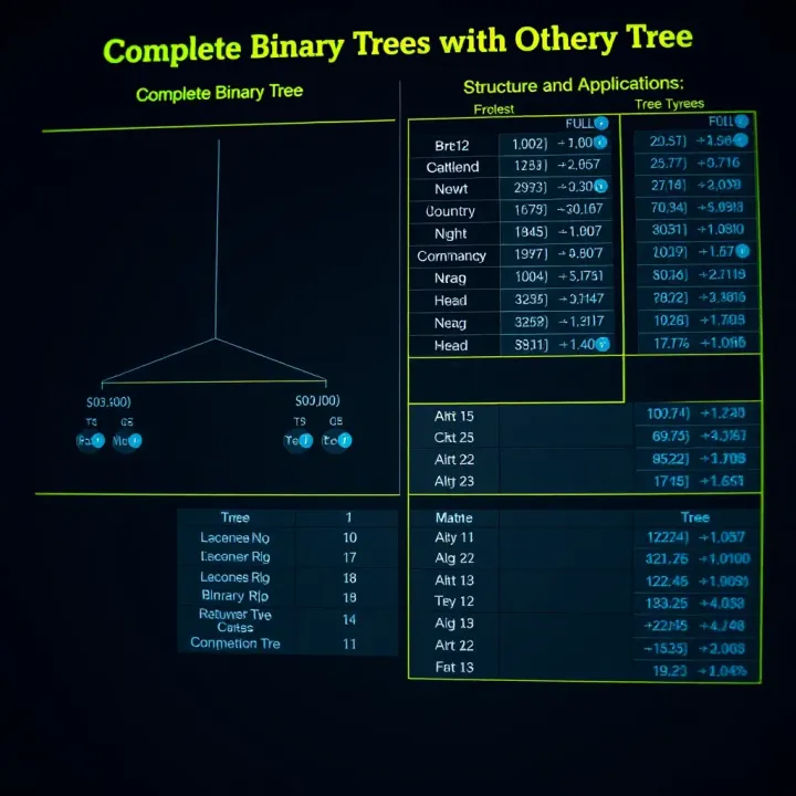
Balanced Height: The height of the tree is minimal for the number of nodes it contains. This means fewer levels and quicker access time.
Node Filling Rule: All levels except the last are completely filled, reducing wasted space compared to other tree types.
Left-align Last Level: Nodes on the last level fill from left to right without gaps, enhancing predictability in data traversal.

A complete binary tree can be efficiently stored as an array since the index relationships between parent and children are straightforward. This allows easy navigations like: for node at index i, the left child is at 2i + 1, the right child at 2i + 2.

Practical Applications

Heaps: Both min-heaps and max-heaps rely on complete binary trees to maintain a balanced and accessible priority structure.
Memory Management: Used in managing memory in operating systems where quick allocation and deallocation are essential.
Networking: Routing tables and hierarchical structures in protocols may use variations of complete trees.

By recognising these properties, programmers and financial analysts can design data systems that are both fast and resource-efficient. Knowing how complete binary trees work helps when dealing with large datasets or real-time processing, such as risk analysis or stock trend computations.

Having a solid grasp of complete binary trees, you can better appreciate why they’re favoured in performance-critical applications compared to other tree types like full or perfect binary trees, which have stricter node requirements but are less flexible in real-world datasets.

Understanding the Structure of a Complete Binary Tree

Diagram illustrating the structure of a complete binary tree showing all levels filled except possibly the last

top

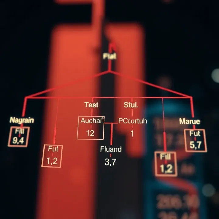
Understanding the structure of a complete binary tree is foundational for grasping many concepts in computer science and data structures. Knowing how nodes are arranged and how the tree fills itself level by level helps optimise algorithms, especially in memory storage and priority queue management. It gives you clarity on why complete binary trees are preferred for certain operations like heaps, where maintaining a balanced but not necessarily perfect structure is crucial.

Definition and Basic Characteristics

A complete binary tree is a binary tree where all levels are fully filled except possibly the last, which is filled from the left up to a point. Imagine a tree where the first few layers are completely packed with nodes, and only the last layer may have some missing nodes but only on the right side. This ensures the tree's shape remains compact, minimizing gaps and making it efficient for storing data sequentially.

This property is practical because it guarantees a minimal height, which improves the speed of operations like insertion and deletion. For example, when you store a complete binary tree in an array, you don’t waste any spaces except possibly at the end, making indexing operations straightforward.

Complete binary trees differ from full and perfect binary trees in their strictness of node arrangements. A full binary tree requires every node to have either zero or two children, which can lead to less dense structures. In contrast, a perfect binary tree is both full and complete, meaning all levels are perfectly filled without any missing nodes.

The complete binary tree relaxes perfection by allowing the last level to be incomplete but insists on filling nodes left to right. This difference is vital in scenarios like heap implementations, where flexibility in the last level avoids unnecessary reorganisation but preserves balance.

Visual Representation

Visualising a complete binary tree helps spot how these rules play out. For instance, try picturing a three-level tree: the first and second levels are fully packed with 1 and 2 nodes respectively, while the third level may have nodes only on the left side, say 3 nodes instead of the full 4 possible. This clear left-to-right filling ensures no random gaps.

In practical terms, each level i (starting from zero) can hold up to 2^i nodes. The tree fills these up one level at a time, and only the last level can be partially filled but only from the left side. This orderly filling means algorithms can depend on position-based calculations, such as computing a parent or child index in arrays without extra pointers, simplifying coding and enhancing performance.

Understanding these visual and structural nuances helps programmers design efficient trees and algorithms, vital in systems handling large datasets or requiring quick access like financial trading platforms or real-time data analysis tools.

Ultimately, the structure of a complete binary tree is what makes it so widely useful, striking the right balance between fullness and flexibility for many computing tasks.

Key Properties of Complete Binary Trees

Understanding the key properties of complete binary trees helps clarify their efficient structure and common uses in computing. These properties influence how nodes are arranged, the height of the tree, and the balance between speed and space during operations.

Node Arrangement and Depth

Nodes in a complete binary tree are arranged layer by layer, filling each level from left to right before moving to the next. This ensures there are no gaps between nodes on any level except possibly the last one. For instance, if a tree has 10 nodes, the first three levels will be fully filled, while the fourth level will have nodes starting from the left without holes until all nodes are placed. This left-to-right placement simplifies operations like insertion because it guarantees a predictable position for new nodes.

This orderly layout also impacts the depth of the tree. The depth is the number of edges from the root to the deepest leaf; by filling levels completely before starting a new one, the tree maintains minimal height, which helps in reducing access time in data structures like heaps.

Maximum Nodes at Each Level

At each level of a complete binary tree, the number of possible nodes doubles compared to the previous level. The root level (level 0) has 1 node, level 1 has a maximum of 2 nodes, level 2 has up to 4 nodes, and so on. This exponential growth continues until the last level, which may not be fully complete but still follows the left-to-right filling rule.

This property means for a tree of height h, the maximum nodes at level i is 2^i. For example, a tree of height 3 can have up to 8 nodes at the last level (level 3). Knowing this helps in calculating memory allocation and understanding how data scales in trees used for priority queues or scheduling.

Height and Number of Nodes

The total number of nodes, N, in a complete binary tree with height h follows a simple formula: 1 + 2 + 4 + + 2^h, which sums to 2^(h + 1) - 1 for a perfect tree. Since a complete binary tree might not have the last level fully filled, the actual node count will be between 2^h and 2^(h + 1) - 1.

This formula helps in estimating the tree's height if you know the number of nodes. For example, if a complete binary tree has 100 nodes, its height h roughly satisfies 2^h ≤ 100 2^(h + 1), so the height is about 6, as 2^6 = 64 and 2^7 = 128.

Calculating Height Based on Node Count

Height calculation is crucial for efficient tree operations because many algorithms depend on the tree’s depth. You can calculate the minimum height, h, of a complete binary tree with N nodes using the formula:

plaintext h = ⌊log₂ N⌋


For instance, if you have 500 nodes, the height will be approximately log₂(500) ≈ 8.96, so the height is 8 when considering integer height levels. This calculation enables programmers to anticipate the worst-case search or insertion times, which are proportional to the height.

> **In practice, complete binary trees balance depth and node distribution efficiently, providing predictable node placement and manageable heights, which is why they are favoured in priority queues and heap implementations.**

These properties together ensure algorithms on complete binary trees perform reliably with time complexity often close to O(log N), making the trees practical for many computing tasks.

## Applications of Complete Binary Trees in Computing

Complete binary trees find critical use in computing, particularly where efficient data organisation and access speed are necessary. Their unique property of being entirely filled except possibly the last level makes them ideal for structures where quick insertion, deletion, and retrieval are required without wasting space.

### Use in Heap Data Structures

Heaps, especially min-heaps and max-heaps, rely heavily on complete binary trees for their structure. A min-heap arranges elements so the smallest is always at the root, while a max-heap keeps the largest at the root. This makes heaps invaluable for priority queue implementations, where the element with the highest or lowest priority must be accessed quickly.

For example, in a min-heap, when a new element is inserted, it is placed in the leftmost available position on the lowest level to maintain completeness. The tree then adjusts by "bubbling up" the element to preserve the heap property. The completeness ensures the tree remains balanced, leading to predictable performance in insertion and removal operations.

Maintaining completeness in heaps ensures the tree height remains logarithmic relative to the number of nodes. This property is essential for priority queues where operations like extracting minimum or maximum elements should work efficiently. Without completeness, tree height could increase, slowing down these critical operations.

### Efficient Memory Storage

One significant advantage of complete binary trees is their natural fit for array representation. Since all levels except possibly the last are full, you can store nodes in a simple array without needing pointers. This method saves memory and improves cache efficiency compared to traditional linked structures.

Array representation avoids the overhead of storing [additional](/articles/understanding-binary-addition/) pointers, which helps in environments with limited memory or where performance is key. For instance, heaps implemented with complete binary trees often store data in arrays where parent-child relationships correspond to index calculations.

Simple indexing is another benefit. Given an element at index *i* in the array, the parent node can be found at index *(i - 1) // 2*, while the children are at indices *2i + 1* and *2i + 2*. This direct calculation eliminates the need for complex pointer traversals, making operations like insertion, deletion, and traversal faster and more straightforward to implement.

> The use of complete binary trees in heaps and their array-based storage shows how understanding tree structures translates directly into practical and efficient computing solutions.

## Algorithms and Operations on Complete Binary Trees

Understanding the algorithms and operations specific to complete binary trees is key for leveraging their structure efficiently. These trees strikingly balance node placement, making operations like insertion, deletion, and traversal both fast and systematic. Practical applications in data structures such as heaps highlight why mastering these operations is essential for traders, analysts, and educators alike.

### Insertion and Deletion Methods

**Maintaining completeness during insertion** is critical because any disruption can turn a complete binary tree into an incomplete one, losing its characteristic shape. Insertions typically happen at the leftmost open position at the lowest level to preserve the tree’s compactness. For example, if you imagine the tree as a near-perfectly filled pyramid, each new element fills the next available space from left to right, leaving no gaps. This approach ensures that when managed in memory or arrays, the indexing remains predictable and efficient.

**Deletion strategies and re-balancing** focus primarily on removing the root or other important nodes without compromising completeness. Usually, the last node (rightmost node at the lowest level) is swapped with the node to be deleted, then removed, maintaining the tree's shape. After this swap, re-balancing using heapify operations restores order in priority queues or heaps. This ensures operations remain O(log n), which is crucial when dealing with large datasets or real-time systems.

### Traversal Techniques

**Inorder, Preorder, Postorder traversals** provide several ways to visit each node, useful for different tasks like searching or expression parsing. In a complete binary tree, these depth-first traversals give a complete sense of node data in different orders. For instance, inorder traversal visits left subtree, node, then right subtree, which is valuable when the tree is also a binary search tree. In financial computing contexts, these traversals help efficiently retrieve data sequences or construct expressions where node order matters.

**Level order traversal and its utility** stands out in complete binary trees because of the tree's structure itself. This traversal visits nodes level by level, from left to right, naturally reflecting how nodes are stored and processed in heaps or queues. It's especially useful when you want to process elements in the exact order they were inserted or are organised—for instance, in breadth-first search or scheduling applications. Level order traversal’s linear approach to processing nodes fits well with array storage, making it efficient in both time and memory.

> Effective algorithms for insertion, deletion, and traversal are the backbone of harnessing the full power of complete binary trees. Their practical relevance extends to dynamic data scenarios and performance-critical applications in Pakistan’s fast-evolving tech and financial sectors.

By understanding and implementing these operations carefully, professionals like traders and analysts can ensure their systems run smoothly with predictable time and memory performance.

## Comparing Complete Binary Trees with Other Tree Types

Understanding how complete binary trees differ from other tree types helps clarify when to use them and what advantages they hold. This comparison is particularly useful for programmers and analysts who seek efficient tree structures for specific applications such as heaps, sorting, or search algorithms.

### Differences from Full and Perfect Binary Trees

**Node completeness vs fullness**: A complete binary tree ensures all levels except possibly the last are fully filled, with nodes as far left as possible. In contrast, a full binary tree demands every node have either two children or none. Practically, completeness focuses on how nodes fill levels from left to right, while fullness focuses on the presence or absence of children per node.

For example, in a full binary tree, it's impossible to have a single child node without its sibling, but a complete tree can have the last level partially filled from the left. This difference matters when maintaining heap structures, where completeness ensures efficient array storage, while fullness doesn’t necessarily impact performance.

**Impacts on tree height and density**: Complete binary trees maintain minimal height given their number of nodes, but may have the last level incomplete. Perfect binary trees, a strict subset, are always fully filled at every level, representing maximum density.

This difference impacts memory and traversal efficiency. Complete trees strike a balance, keeping height low to reduce search or update time, while being flexible enough for partial filling at the bottom. This results in a compact structure that’s easier to manage in memory compared to less strictly organised trees.

### Relation to Binary Search Trees and Balanced Trees

**Structural differences**: Binary Search Trees (BST) organise nodes based on key values, so left children contain smaller values and right children larger ones. Complete binary trees enforce node positioning based on filling order rather than value, ignoring the BST property.

Balanced trees, such as AVL or Red-Black trees, maintain strict height constraints to ensure operations stay fast, but their node filling isn’t left-to-right complete. Complete binary trees have fixed level filling but no inherent order among node values.

This structural distinction means complete binary trees are suited for uses where shape matters, like heaps, but aren’t ideal for direct searching since they lack ordered traversal paths.

**Suitability for various algorithms**: Algorithms needing quick insertion, deletion, or priority access benefit from complete binary trees due to their compactness and array-based representation. Heap operations rely on the complete tree property to efficiently maintain priorities.

On the other hand, searching algorithms and range queries rely on BSTs or balanced trees for value ordering, which complete binary trees don’t provide. Therefore, choosing a tree type depends on whether you prioritise insertion speed and memory efficiency or value-based searching.

> In practical terms, understanding these differences guides you toward the right data structure, making operations more efficient and simpler in systems ranging from database indexing to network routing tables.